Droplet Breakup

Files

File	Description
input.sdf	Input file

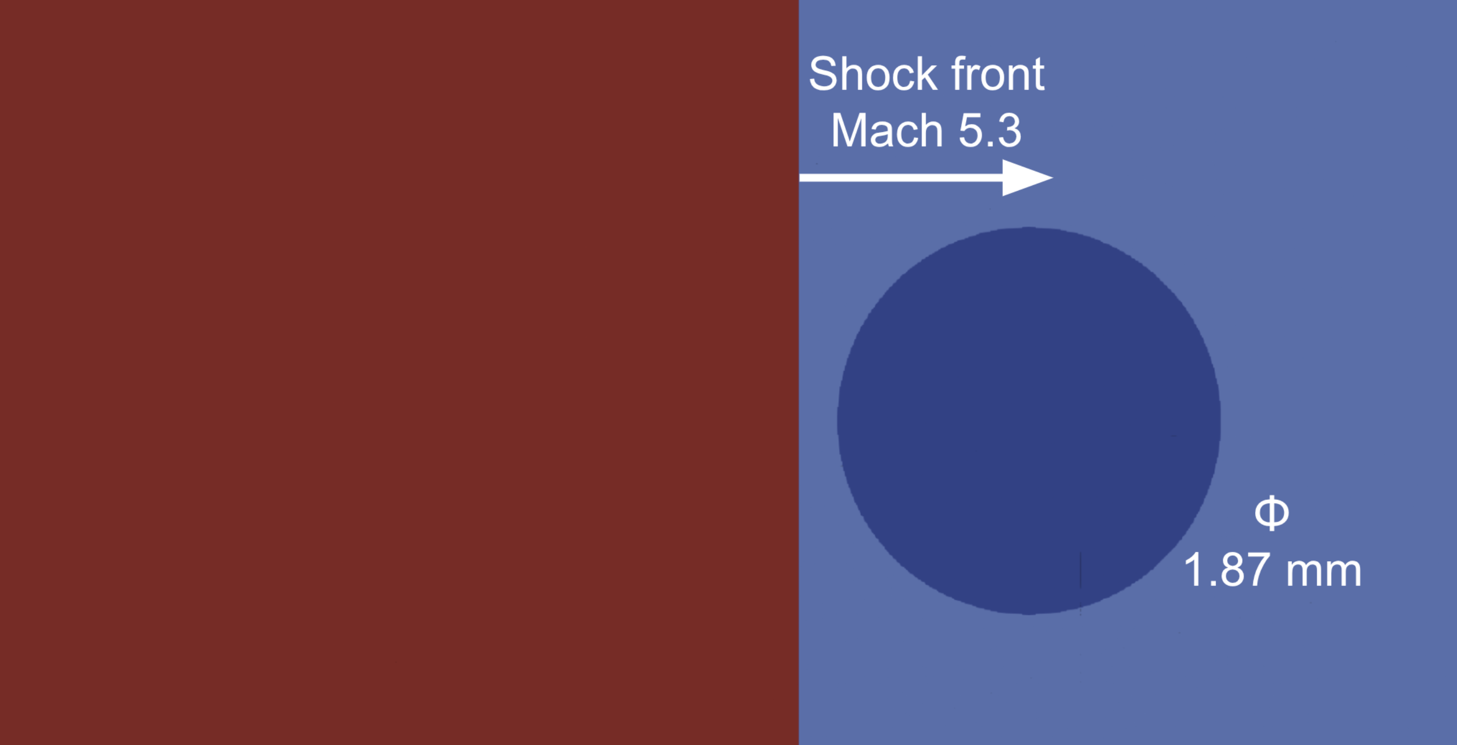Initial configuration of the aero-breakup case: a planar shock advancing toward a spherical liquid droplet.

Introduction

Installation required

This tutorial assumes you've followed the installation instructions.

This is a multiphase test case for spherical droplet aero-breakup at Mach 5.3, with a droplet diameter of 1.87 mm. A liquid droplet (density 1000 kg/m³) sits in quiescent air at atmospheric pressure, with a planar shock wave positioned just upstream, moving at a shock Mach number of $M_s \approx 5.30$. This follows from the normal-shock pressure-ratio relation

$\frac{P_2}{P_1} = \frac{2\gamma M_s^2 - (\gamma - 1)}{\gamma + 1}$

evaluated with the pre- and post-shock pressures set in the initial condition (P1, P2) and $\gamma = \gamma_{gas} = 1.3$. As the simulation proceeds, the shock sweeps over the droplet and triggers aerodynamic breakup: deformation, stripping, and fragmentation of the liquid volume.

This case is also a good illustration of the Dictionary block as a preprocessing facility: rather than hardcoding values throughout the file, quantities like the droplet geometry (ddmaj, ddmin), grid spacing (dxmin), and shock location (shockloc) are defined once as expressions in terms of a small set of base parameters, then reused wherever needed — including inside the analytic InitialCondition and Refinement expressions later in the file. Changing a single base parameter (e.g. ppd or xd) propagates consistently everywhere it's used.

Dictionary keys are freeform

Dictionary isn't a fixed schema — unlike blocks such as Domain or Integration, it doesn't have a required set of keys. You can define any key names you like, as plain numbers or as expressions referencing other keys defined above them. A key only does anything if it's actually referenced elsewhere — in another Dictionary expression, or in a string expression inside a block like InitialCondition or Refinement; an unreferenced key is just inert. That's what makes Dictionary useful as a parameterization layer: define a case's "knobs" once at the top, under whatever names make sense, then reference them everywhere they're needed throughout the rest of the file. It is recommended to have as few dictionary parameters as you need to run the simulation that you are interested in.

Case Summary

Quantity	Value
Shock Mach number	$M_s \approx 5.30$
Droplet diameter ($D$)	1.87 mm
Initial grid size	$\approx$ 213.2 million cells
Minimum grid spacing ($\Delta x$)	6.09 μm
$\Delta x / D$	$\approx 3.26 \times 10^{-3}$ (≈ 307 cells across the droplet diameter)

Getting Started

To run this case, simply invoke:

champs+ input.sdf

If you have multiple GPUs available and want to distribute the run across, say, two of them:

champs+ -dev 0,1 input.sdf

Command line reference

See the command line reference for the full set of available flags, including other device-selection options.

Running the case creates a sim/ output directory (set by IO::output_directory) with the following structure:

sim/
  log/       solver log files
  restart/   binary .db checkpoint files, written every Restart::output_interval seconds; usable to restart another simulation
  slice/
    slice_z/   the z = 0 plane output defined under IO::Outputs::slice_z, written every 0.2 μs — open the .vtm files in ParaView
  _cache/
  _comm/
  _debug/

Subdirectories prefixed with an underscore are used internally by the solver and can generally be ignored — the results you care about are in log/, restart/, and slice/.

Results

This tutorial is primarily a visual check — run the case to completion and compare your slice_z output against the figures below.

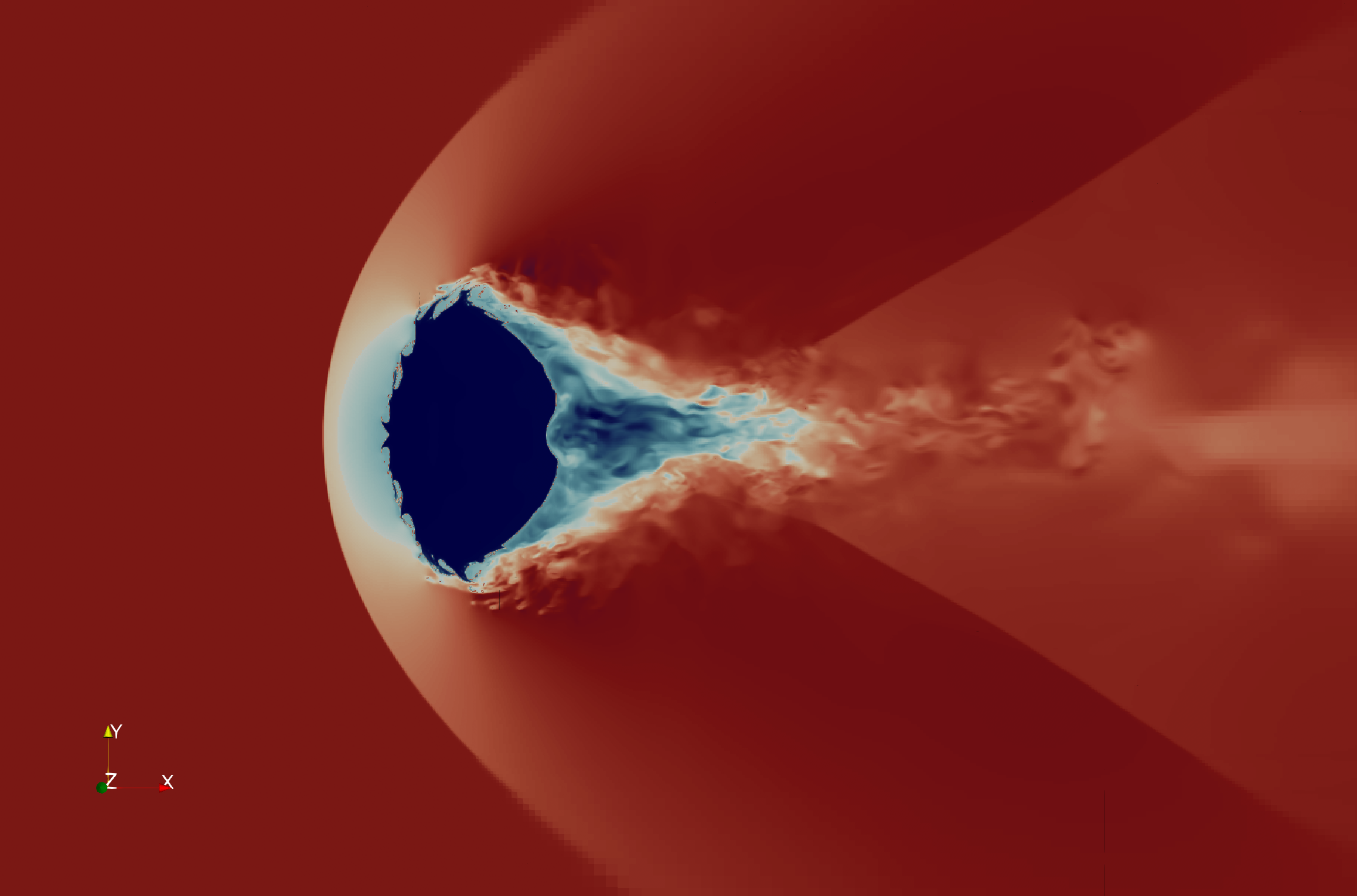Symmetry-plane (z = 0) slice showing the bow shock standing off the droplet, the deformed liquid core, and stripped liquid mist trailing into the wake.

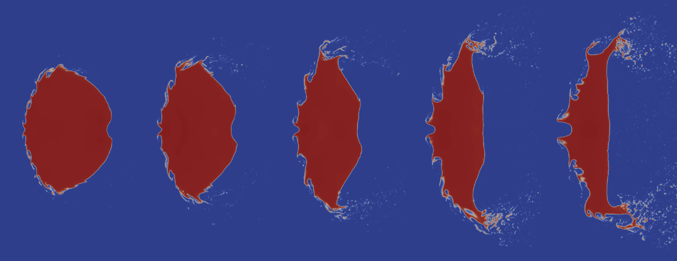Evolution of the droplet shape over the course of the simulation: the initially spherical droplet flattens, then progressively deforms and fragments at its edges as it's swept downstream.

You should see the same overall progression in your own run: a bow shock forms ahead of the droplet, the droplet flattens into a disk-like shape, and its edges begin to strip and fragment as the flow develops.

Grid Resolution

The grid resolution for this case is controlled by a single Dictionary parameter, ppd — points per (droplet) diameter. It sets the finest target cell spacing, dxmin:

$\Delta x_{min} = \frac{2 \cdot ddmin}{ppd} = \frac{D}{ppd}$

ddmin  = 0.00187/2
ddmaj  = 0.00187/2
dxmin  = ddmin*2/ppd

dxmin is then used directly as the target spacing for both the base grid and the finest static refinement level:

Domain
{
    Grid
    {
        dx_target = [dxmin, dxmin, dxmin]
        ...
        Refinement
        {
            Spacing
            {
                dx_base   = [dxmin,   dxmin,   dxmin]
                dx_coarse = [2*dxmin, 2*dxmin, 2*dxmin]
            }

Since dxmin is defined in terms of ppd in the Dictionary, increasing ppd and rerunning is enough to refine the whole case — every expression that depends on dxmin picks up the change automatically, no other edits needed.

The table below shows the achieved spacing and resulting initial grid size (from the static base_patch/coarse_patch refinement, before any AMR) for a few values of ppd, taken from solver log output:

ppd	Target $\Delta x$	Achieved $\Delta x$	$D / \Delta x$	Initial grid size
100	18.7 μm	18.26 μm	102.4	12,061,440
200	9.35 μm	9.13 μm	204.8	76,799,232
300	6.23 μm	6.09 μm	307.2	213,153,984

Grid size grows faster than linearly with ppd — going from ppd=100 to ppd=300 (3×) grows the initial grid by roughly 18×, not 3× — since the entire refined region around the droplet is resolved volumetrically. Increase ppd gradually and keep an eye on grid size and available GPU memory before committing to a large run.

Other Variations

Shock strength (Mach number)

Shock strength isn't a single Mach number parameter in this file — P2, R2, T2, and u2lf (used as Qinf::uinf) together define the post-shock state, and must be changed as a self-consistent set using the same normal-shock relations that gave $M_s \approx 5.30$ in the Introduction:

$\frac{P_2}{P_1} = \frac{2\gamma M_s^2 - (\gamma - 1)}{\gamma + 1}, \qquad \frac{R_2}{R_1} = \frac{(\gamma+1) M_s^2}{(\gamma-1)M_s^2 + 2}, \qquad u_2 = \frac{2 a_1}{\gamma + 1}\left(M_s - \frac{1}{M_s}\right)$

where $a_1 = \sqrt{\gamma_{gas} P_1 / R_1}$ is the ambient sound speed and $\gamma = \gamma_{gas}$. To target a new $M_s$: compute P2 and R2 from P1/R1 with the relations above, set u2lf to the resulting $u_2$, and get T2 from the ideal gas law, $T_2 = P_2 / (R_2 \cdot R_{gas})$.

Droplet size and shape

Droplet geometry is set by ddmaj (streamwise, x-direction) and ddmin (transverse, y/z) in the Dictionary — currently equal, giving a 1.87 mm sphere. Because grid spacing (dxmin), the domain bounds, and every refinement zone are all expressed in terms of ddmin/ddmaj, resizing the droplet (e.g. ddmin = ddmaj = 0.003/2) rescales the whole case automatically at the same relative resolution (ppd) and domain proportions, with no other edits needed. Setting ddmaj != ddmin instead produces an ellipsoidal droplet, since the InitialCondition expressions use ddmaj2 for the x-extent and ddmin2 for the y/z extent.