Getting Started

Files

File	Description
input.sdf	Input file
cone.vtk	Triangulation for the blunt cone geometry

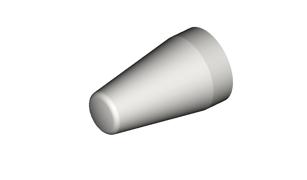Geometry of the blunted cone forebody used in this case.

Introduction

Installation required

This tutorial assumes you've followed the installation instructions.

This is an inviscid, hypersonic test case: uniform Mach 6 flow over a blunted cone at a 12.5° angle of attack, based on the forebody geometry from NASA TN D-1790 (Holloway & Dunavant, 1963). The cone surface is given as a triangulated cone.vtk geometry and represented on the Cartesian grid using the immersed boundary method (IBM), with a slip-wall boundary condition. Time-accurate explicit time integration is used.

Case Summary

Quantity	Value
Freestream Mach number	6
Angle of attack	12.5°
Freestream pressure ($P_\infty$)	10 kPa
Freestream temperature ($T_\infty$)	100 K
Initial grid size	$\approx$ 15.9 million cells
Minimum grid spacing ($\Delta x$)	$\approx$ 967 μm (target 1 mm)

Running the Case

To run this case, simply invoke:

champs+ input.sdf

If you have multiple GPUs available and want to distribute the run across, say, two of them:

champs+ -dev 0,1 input.sdf

Command line reference

See the command line reference for the full set of available flags, including other device-selection options.

The case runs for max_steps = 13000 steps (Integration::max_steps) at CFL = 0.45 using explicit ssprk3 time integration. On a single GPU, expect this case to run in 4-10 minutes.

Running the case creates a sim/ output directory (set by IO::output_directory) with the following structure:

sim/
  log/            solver log files
  restart/        binary .db checkpoint files, written every Restart::output_interval steps (1000); usable to restart another simulation
  slice/
    sym_plane/    the z = 0.001 symmetry-plane slice defined under IO::Outputs::sym_plane, written every 1000 steps — open the .vtm files in ParaView
  surface/
    surf_out/     body-surface fields defined under IO::Outputs::surf_out, written every 1000 steps — .vtk files, open in ParaView
  profile/
    press_out/    pressure/Cp profile CSVs defined under IO::Outputs::press_out, written every 1000 steps
  _cache/         used internally by the solver
  _comm/          used internally by the solver
  _debug/         used internally by the solver

Subdirectories prefixed with an underscore are used internally by the solver and can generally be ignored — the results you care about for this case are in log/, restart/, slice/, surface/, and profile/.

Results

Run the case to completion and compare your sym_plane slice output against the figures below.

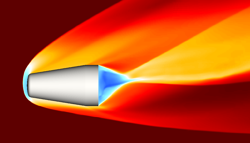Symmetry-plane slice of $M_x$ (streamwise Mach number): a bow shock stands off the blunted nose, with a subsonic pocket (blue) near the tip and in the wake.

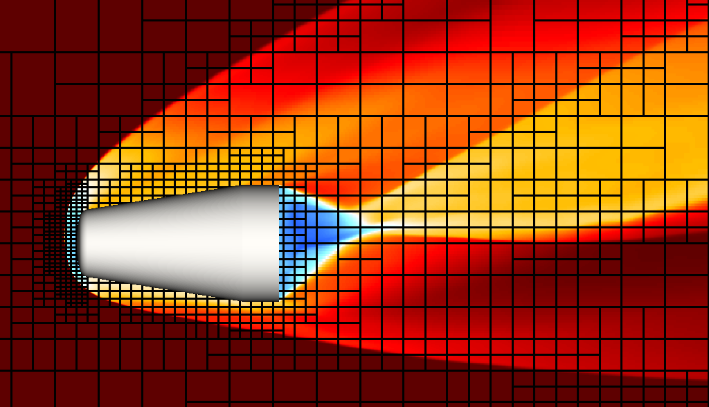The same slice with grid blocks overlaid: spacing is finest at the nose, coarser over the rest of the body, and refined again along the bow shock, courtesy of the nose/body/shock Refinement::Spacing levels and the AMR criterion tracking pressure.

Computing Mach number

The sym_plane slice only exports the primitive variables {P, T, U, V, W} — Mach number isn't written out directly. Compute it in your postprocessing tool of choice (Tecplot, ParaView, VisIt, ...) as $M = |\mathbf{U}|/\sqrt{\gamma R T}$.

The Input File

Let's walk through input.sdf from top to bottom to see how this case is put together.

Dictionary

Dictionary
{
    Tref     = 100.0
    gamma    = 1.4
    Rgas     = 287.15
    mach     = 6
    aoa      = 12.5
    umag     = mach*sqrt(gamma*Rgas*Tref)
    Lscale   = 1.0
    dxmin    = 0.001
    Qinf
    {
        pinf     = 10000.0
        Tinf     = Tref
        uinf     = umag*cos(aoa*#pi/180.0)
        vinf     = umag*sin(aoa*#pi/180.0)
        winf     = 0.0
        rhoinf   = Qinf::pinf/(Rgas*Tref)
    }
}

Dictionary keys are freeform

Dictionary isn't a fixed schema — unlike blocks such as Domain or Integration, it doesn't have a required set of keys. You can define any key names you like, as plain numbers or as expressions referencing other keys defined above them. A key only does anything if it's actually referenced elsewhere — in another Dictionary expression, or in a string expression inside a block like InitialCondition or Refinement; an unreferenced key is just inert. That's what makes Dictionary useful as a parameterization layer: define a case's "knobs" once at the top, under whatever names make sense, then reference them everywhere they're needed throughout the rest of the file. It is recommended to have as few dictionary parameters as you need to run the simulation that you are interested in.

None of these keys are mandatory — they only do anything because they're referenced by name later in the file. Here, the Dictionary is used to front-load the basic gas-dynamics calculations, so the rest of the input file can be written in terms of physically meaningful case parameters instead of raw numbers:

• Tref, gamma, and Rgas set the reference gas state and ideal-gas constant.
• mach and aoa are the two real "knobs" of this case — freestream Mach number and angle of attack.
• umag computes the freestream speed from mach via $u = M\sqrt{\gamma R T}$.
• Lscale is a characteristic length, used further down to define the simulation's characteristic time in Integration.
• dxmin is the target minimum grid spacing, used further down in Domain::Grid.
• The nested Qinf group resolves umag into Cartesian velocity components using aoa ($u_\infty = u\cos\alpha$, $v_\infty = u\sin\alpha$), and computes the freestream density rhoinf from the ideal gas law.

Because uinf, vinf, and rhoinf are all expressed in terms of mach, aoa, and the reference gas properties, changing mach or aoa and rerunning is enough to retarget the whole case to a new flow condition — every place that references Qinf::uinf, Qinf::vinf, etc. later in the file (the InitialCondition and DomainBC blocks) picks up the change automatically.

Geometries

Geometries
{
    cone
    {
        is_external = true
        filename    = "cone.vtk"
        Patches
        {
            nose = ["0", "4"]
        }
        Transforms
        {
            scale
            {
                specifier = "scale"
                scales    = [0.001, 0.001, 0.001] 
            }
        }
    }
}

This defines a single geometry, cone, loaded from the triangulated surface file cone.vtk. See the Geometries reference for the full schema.

• is_external = true tells the solver that flow is external to the body, as opposed to internal (e.g. duct/pipe) flow.
• Patches assigns a human-readable name to a subset of the surface, by id, for use elsewhere in the file. Here, nose = ["0", "4"] groups two surface components from the source file into a single named region, nose.

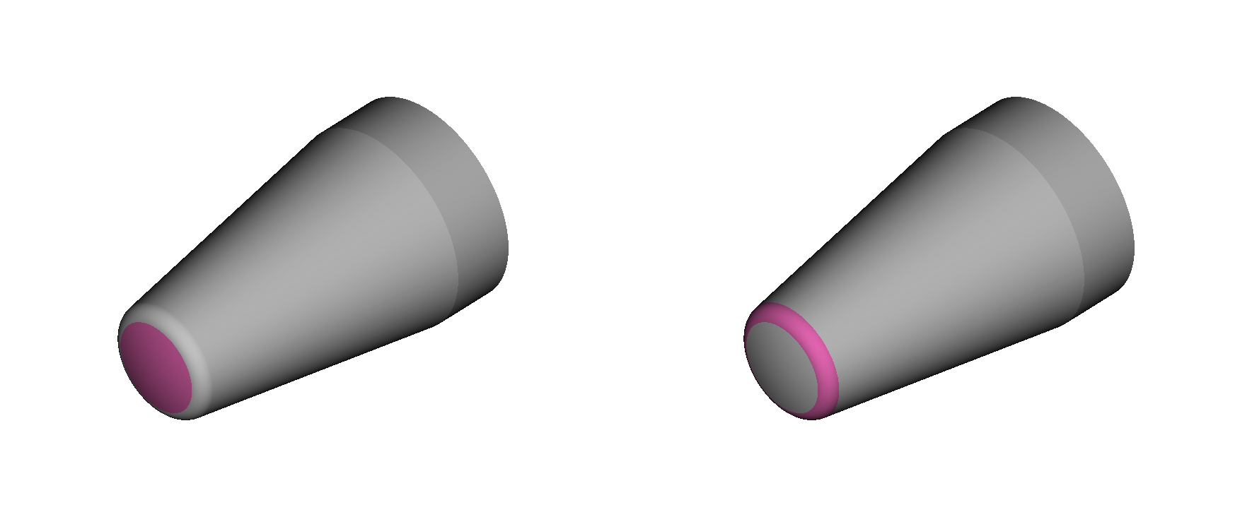Surface components "0" (left) and "4" (right) from cone.vtk: together they make up the rounded nose cap, tangent to the rest of the conical body.

Exactly how these component ids come out of the CAD/mesh export isn't something you need to worry about for this tutorial. What matters is the mechanism: once a set of faces is grouped under a Patches name, that name can be referenced anywhere else in the input file — which is exactly what happens later on, when nose is used to target the finest static refinement level onto just this region.

• Transforms applies an ordered list of transformations to the geometry — see the Transforms reference for the other available specifiers (translate, rotate). Here there's a single scale transform, [0.001, 0.001, 0.001], converting cone.vtk's native units — millimeters — into the meters used throughout the rest of the input file.