Inviscid Simulation
This tutorial walks you through an external, inviscid simulation of a blunted cone at Mach 6 with angle of attack 12.5°. There are three outputs: a symmetry-plane slice, body-surface fields, and a pressure/Cp profile near the symmetry line.
For original test data and figures, see NASA TN D-1790 (Holloway & Dunavant, 1963).
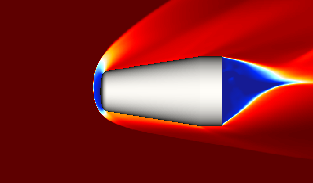 Flowfield (U-velocity) at Mach 6, α = 12.5°; symmetry-plane slice showing bow-shock stand-off and forebody structure.
Running the case
Assuming the champs+ engine is on your path and you have a valid
license file in the directory pointed to by CHAMPS_DATA, you can invoke the engine by simply typing champs+ on the command line. The engine
will default to running the parameters in input.sdf, but if you want to run another input file you can simply run using champs+ other_input.sdf.
See the command line reference for more information on command-line options.
Relevant input options
1) Dictionary
See dictionary.
- Change angle of attack with
aoa; change freestream Mach withmach. dxminsets the target minimum spacing.Lscale = 1.0defines the characteristic length; the characteristic time istc = Lscale/umag.
2) Integration
See integration.
- Run for 5 characteristic times (stop time ≈
5*tc). This is typically enough to settle a supersonic inviscid simulation.
3) IO
-
output_directory = simmeans that all data resulting from this simulation will be in thesimdirectory. -
sym_plane (slice)
- Plane normal
direction = 2atposition = 0.001(slight offset from symmetry). output_interval = 1000steps (output written every 1000 steps).- Use this to check bow-shock location and thickness.
- Plane normal
-
surf_out (surface)
- Writes body surface fields for stagnation pressure/Cp footprints.
- Same cadence (
output_interval = 1000).
-
press_out (profile)
- A
surface_sliceon the body near the symmetry line:point = [0,0,0.001],normal = [0,0,1]. - Exports:
P,Cp = (P − Qinf::pinf)/(0.5*Qinf::rhoinf*umag^2),U,T: these expressions include flowfield values (P,T,U,V,W) and dictionary values.
- A
What to expect
Results from this case should approximately match the provided reference data. There is a python script included
in the tutorial case called plot.py, which can be run using python3 plot.py.


Example comparison of Cp along the symmetry meridian: solver (solid) vs. reference from TN D-1790 (dashed).